TensorFlow-VGG16模型复现

VGG介绍

VGG全称是指牛津大学的Oxford Visual Geometry Group，该小组在2014年的ImageNet挑战赛中，设计的VGG神经网络模型在定位和分类跟踪比赛中分别取得了第一名和第二名的成绩。

• VGG论文

  VERY DEEP CONVOLUTIONAL NETWORKS FOR LARGE-SCALE IMAGE RECOGNITION

论文指出其主要贡献在于：利用3*3小卷积核的网络结构对逐渐加深的网络进行全面的评估，结果表明加深网络深度到16至19层可极大超越前人的网络结构。

VGG结构特点

• 训练输入：固定尺寸224*224的RGB图像
• 预处理：每个像素值减去训练集上的RGB均值
• 卷积核：一系列3*3卷积核堆叠，步长为1，采用padding保持卷积后图像空间分辨率不变
• 空间池化：紧随卷积“堆”的最大池化，为2*2滑动窗口，步长为2
• 全连接层：特征提取完成后，接三个全连接层，前两个为4096通道，第三个为1000通道，最后是一个soft-max层，输出概率
• 所有隐藏层都用非线性修正ReLu

详细配置

表中每列代表不同的网络，只有深度不同（层数计算不包含池化层）。卷积的通道数量很小，第一层仅64通道，每经过一次最大池化，通道数翻倍，直到数量达到512通道。
对比每种模型的参数数量，尽管网络加深，但权重并未大幅增加，因为参数量主要集中在全连接层。
最后两列（D列和E列）是效果较好的VGG-16和VGG-19的模型结构，本文将用TensorFlow代码复现VGG-16模型，并使用训练好的模型参数文件进行图片物体分类测试。

ConvNet Configuration
A	A-LRN	B	C	D	E
11 weight layers	11 weight layers	13 weight layers	16 weight layers	16 weight layers	19 weight layers
Number of parameters(in millions)
133	133	133	134	138	144
input(224x224 RGB image)
conv3-64	conv3-64 LRN	conv3-64 conv3-64	conv3-64 conv3-64	conv3-64 conv3-64	conv3-64 conv3-64
maxpool
conv3-128	conv3-128	conv3-128 conv3-128	conv3-128 conv3-128	conv3-128 conv3-128	conv3-128 conv3-128
maxpool
conv3-256 conv3-256	conv3-256 conv3-256	conv3-256 conv3-256	conv3-256 conv3-256 conv1-256	conv3-256 conv3-256 conv3-256	conv3-256 conv3-256 conv3-256 conv3-256
maxpool
conv3-512 conv3-512	conv3-512 conv3-512	conv3-512 conv3-512	conv3-512 conv3-512 conv1-512	conv3-512 conv3-512 conv3-512	conv3-512 conv3-512 conv3-512 conv3-512
maxpool
conv3-512 conv3-512	conv3-512 conv3-512	conv3-512 conv3-512	conv3-512 conv3-512 conv1-512	conv3-512 conv3-512 conv3-512	conv3-512 conv3-512 conv3-512 conv3-512
maxpool
FC-4096
FC-4096
FC-1000
soft-max

论文中介绍的训练方法

• 训练方法基本与AlexNet一致，除了多尺度训练图像采样方法不一致
• 训练采用mini-batch梯度下降法，batch size=256
• 采用动量优化算法，momentum=0.9
• 采用L2正则化方法，惩罚系数0.00005，dropout比率设为0.5
• 初始学习率为0.001，当验证集准确率不再提高时，学习率衰减为原来的0.1倍，总共下降三次
• 总迭代次数为370K（74epochs）
• 数据增强采用随机裁剪，水平翻转，RGB颜色变化
• 设置训练图片大小的两种方法（定义S代表经过各向同性缩放的训练图像的最小边）：
  • 第一种方法针对单尺寸图像训练，S=256或384，输入图片从中随机裁剪224*224大小的图片，原则上S可以取任意不小于224的值
  • 第二种方法是多尺度训练，每张图像单独从[Smin ,Smax ]中随机选取S来进行尺寸缩放，由于图像中目标物体尺寸不定，因此训练中采用这种方法是有效的，可看作一种尺寸抖动的训练集数据增强

论文中提到，网络权重的初始化非常重要，由于深度网络梯度的不稳定性，不合适的初始化会阻碍网络的学习。因此先训练浅层网络，再用训练好的浅层网络去初始化深层网络.

VGG-16网络复现

VGG-16网络结构(前向传播)复现

复现VGG-16的16层网络结构，将其封装在一个Vgg16类中，注意这里我们使用已训练好的vgg16.npy参数文件，不需要自己再对模型训练，因而不需要编写用于训练的反向传播函数，只编写用于测试的前向传播部分即可。

下面代码我已添加详细注释，并添加一些print语句用于输出网络在每一层时的结构尺寸信息。

vgg16.py

import inspect
import os
import numpy as np
import tensorflow as tf
import time
import matplotlib.pyplot as plt

VGG_MEAN = [103.939, 116.779, 123.68] # 样本RGB的平均值

class Vgg16():
    def __init__(self, vgg16_path=None):
        if vgg16_path is None:
            # os.getcwd()方法用于返回当前工作目录(npy模型参数文件)
            vgg16_path = os.path.join(os.getcwd(), "vgg16.npy")
            print("path(vgg16.npy):",vgg16_path)
            # 遍历其内键值对，导入模型参数
            self.data_dict = np.load(vgg16_path, encoding='latin1').item()
        for x in self.data_dict: # 遍历datat_dict中的每个键
            print("key in data_dict:",x)

    def forward(self, images):
        
        print("build model started...")
        start_time = time.time() # 获取前向传播的开始时间  
        rgb_scaled = images * 255.0 # 逐像素乘以255
        # 从GRB转换色彩通道到BGR
        red, green, blue = tf.split(rgb_scaled,3,3)
        # assert是加入断言，用断每个操作后的维度变化是否和预期一致
        assert red.get_shape().as_list()[1:] == [224, 224, 1]
        assert green.get_shape().as_list()[1:] == [224, 224, 1]
        assert blue.get_shape ().as_list()[1:] == [224, 224, 1]
        
        bgr = tf.concat([     
            blue - VGG_MEAN[0],
            green - VGG_MEAN[1],
            red - VGG_MEAN[2]],3)
        assert bgr.get_shape().as_list()[1:] == [224, 224, 3]

        #构建VGG的16层网络（包含5段(2+2+3+3+3=13)卷积，3层全连接）
        # 第1段，2卷积层+最大池化层
        print("==>input image shape:",bgr.get_shape().as_list())
        self.conv1_1 = self.conv_layer(bgr, "conv1_1")
        print("=>after conv1_1 shape:",self.conv1_1.get_shape().as_list())
        self.conv1_2 = self.conv_layer(self.conv1_1, "conv1_2")
        print("=>after conv1_2 shape:",self.conv1_2.get_shape().as_list())
        self.pool1 = self.max_pool_2x2(self.conv1_2, "pool1")
        print("---after pool1 shape:",self.pool1.get_shape().as_list())

        # 第2段，2卷积层+最大池化层
        self.conv2_1 = self.conv_layer(self.pool1, "conv2_1")
        print("=>after conv2_1 shape:",self.conv2_1.get_shape().as_list())
        self.conv2_2 = self.conv_layer(self.conv2_1, "conv2_2")
        print("=>after conv2_2 shape:",self.conv2_2.get_shape().as_list())
        self.pool2 = self.max_pool_2x2(self.conv2_2, "pool2")
        print("---after pool2 shape:",self.pool2.get_shape().as_list())

        # 第3段，3卷积层+最大池化层
        self.conv3_1 = self.conv_layer(self.pool2, "conv3_1")
        print("=>after conv3_1 shape:",self.conv3_1.get_shape().as_list())
        self.conv3_2 = self.conv_layer(self.conv3_1, "conv3_2")
        print("=>after conv3_2 shape:",self.conv3_2.get_shape().as_list())
        self.conv3_3 = self.conv_layer(self.conv3_2, "conv3_3")
        print("=>after conv3_3 shape:",self.conv3_3.get_shape().as_list())
        self.pool3 = self.max_pool_2x2(self.conv3_3, "pool3")
        print("---after pool3 shape:",self.pool3.get_shape().as_list())

        # 第4段，3卷积层+最大池化层
        self.conv4_1 = self.conv_layer(self.pool3, "conv4_1")
        print("=>after conv4_1 shape:",self.conv4_1.get_shape().as_list())
        self.conv4_2 = self.conv_layer(self.conv4_1, "conv4_2")
        print("=>after conv4_2 shape:",self.conv4_2.get_shape().as_list())
        self.conv4_3 = self.conv_layer(self.conv4_2, "conv4_3")
        print("=>after conv4_3 shape:",self.conv4_3.get_shape().as_list())
        self.pool4 = self.max_pool_2x2(self.conv4_3, "pool4")
        print("---after pool4 shape:",self.pool4.get_shape().as_list())

        # 第5段，3卷积层+最大池化层
        self.conv5_1 = self.conv_layer(self.pool4, "conv5_1")
        print("=>after conv5_1 shape:",self.conv5_1.get_shape().as_list())
        self.conv5_2 = self.conv_layer(self.conv5_1, "conv5_2")
        print("=>after conv5_2 shape:",self.conv5_2.get_shape().as_list())
        self.conv5_3 = self.conv_layer(self.conv5_2, "conv5_3")
        print("=>after conv5_3 shape:",self.conv5_3.get_shape().as_list())
        self.pool5 = self.max_pool_2x2(self.conv5_3, "pool5")
        print("---after pool5 shape:",self.pool5.get_shape().as_list())

        # 3层全连接层
        self.fc6 = self.fc_layer(self.pool5, "fc6") # 输出4096长度
        print("=>after fc6 shape:",self.fc6.get_shape().as_list())
        assert self.fc6.get_shape().as_list()[1:] == [4096]
        self.relu6 = tf.nn.relu(self.fc6)         
        self.fc7 = self.fc_layer(self.relu6, "fc7")
        print("=>after fc7 shape:",self.fc7.get_shape().as_list())
        self.relu7 = tf.nn.relu(self.fc7)        
        self.fc8 = self.fc_layer(self.relu7, "fc8")
        print("=>after fc8 shape:",self.fc8.get_shape().as_list())

        # softmax分类，得到属于各类别的概率
        self.prob = tf.nn.softmax(self.fc8, name="prob")
        
        end_time = time.time() # 得到前向传播的结束时间  
        print(("forward time consuming: %f" % (end_time-start_time)))

        # 清空本次读取到的模型参数字典
        self.data_dict = None 

    # 定义卷积运算   
    def conv_layer(self, x, name):
        # 根据命名空间name从参数字典(npy文件)中取到对应卷积层的网络参数
        with tf.variable_scope(name): 
            w = self.get_conv_filter(name) # 读到该层的卷积核大小
            # 卷积计算
            conv = tf.nn.conv2d(x, w, [1, 1, 1, 1], padding='SAME') 
            conv_biases = self.get_bias(name) # 读到偏置项b
            # 加上偏置，并做激活计算
            result = tf.nn.relu(tf.nn.bias_add(conv, conv_biases)) 
            return result

    # 定义获取卷积核大小的函数
    def get_conv_filter(self, name):
        # 根据命名空间name从参数字典中取到对应的卷积核大小
        return tf.constant(self.data_dict[name][0], name="filter") 

    # 定义获取偏置的函数
    def get_bias(self, name):
        # 根据命名空间name从参数字典中取到对应的偏置
        return tf.constant(self.data_dict[name][1], name="biases")

    # 定义2x2最大池化操作
    def max_pool_2x2(self, x, name):
        return tf.nn.max_pool(x, ksize=[1, 2, 2, 1], strides=[1, 2, 2, 1], padding='SAME', name=name)

    # 定义全连接层的前向传播计算
    def fc_layer(self, x, name):
        # 根据命名空间name做全连接层的计算 
        with tf.variable_scope(name): 
            shape = x.get_shape().as_list() # 获取该层的维度信息列表
            print("fc_layer shape:",shape)
            dim = 1
            for i in shape[1:]:
                dim *= i # 将每层的维度相乘
            #  改变特征图的形状，将得到的多维特征做拉伸操作，只在进入第六层全连接层做该操作
            x = tf.reshape(x, [-1, dim])
            w = self.get_fc_weight(name) # 读到权重值
            b = self.get_bias(name) # 读到偏置项

            # 对该层输入做加权求和，再加上偏置    
            result = tf.nn.bias_add(tf.matmul(x, w), b) 
            return result

    # 定义获取权重的函数
    def get_fc_weight(self, name):
        # 根据命名空间name从参数字典中取到对应的权重
        return tf.constant(self.data_dict[name][0], name="weights")

图片加载显示与预处理

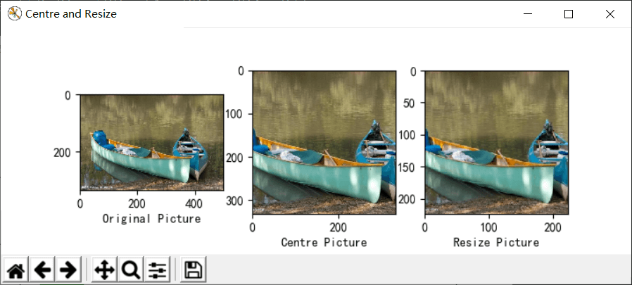
测试图片需要进行必要的预处理操作（尺寸裁剪，像素归一化等），并使用matplotlib将原始图片以及预处理用于测试的图片显示出来。

utils.py

from skimage import io, transform
import numpy as np
import matplotlib.pyplot as plt
import tensorflow as tf
from pylab import mpl

mpl.rcParams['font.sans-serif']=['SimHei'] # 正常显示中文标签
mpl.rcParams['axes.unicode_minus']=False # 正常显示正负号

# 定义加载图像、显示与预处理函数
def load_image(path):
    fig = plt.figure("Centre and Resize")
    img = io.imread(path)  # 根据传入的路径读入图片
    img = img / 255.0 # 将像素归一化到[0,1]

    # 将该画布分为一行三列
    ax0 = fig.add_subplot(131) # 把下面的图像放在该画布的第一个位置   
    ax0.set_xlabel(u'Original Picture')  # 添加子标签
    ax0.imshow(img)  # 添加展示该图像
    
    short_edge = min(img.shape[:2]) # 找到该图像的最短边
    y = (img.shape[0] - short_edge) // 2 
    x = (img.shape[1] - short_edge) // 2  # 把图像的w和h分别减去最短边，求平均
    crop_img = img[y:y+short_edge, x:x+short_edge] # 取出切分出的中心图像
    
    ax1 = fig.add_subplot(132) 
    ax1.set_xlabel(u"Centre Picture") 
    ax1.imshow(crop_img) # 显示中心图像

    # resize成固定的imag_szie224x224
    re_img = transform.resize(crop_img, (224, 224)) 
    
    ax2 = fig.add_subplot(133) 
    ax2.set_xlabel(u"Resize Picture") 
    ax2.imshow(re_img) # 显示224x224图像
	
    img_ready = re_img.reshape((1, 224, 224, 3))

    return img_ready

# 定义百分比转换函数
def percent(value):
    return '%.2f%%' % (value * 100)

物体种类列表

此文件保存1000中预测结果编号对应的真实物体的名称，用于将最后的预测id对应为物体名称。

Nclasses.py

# 每个图像的真实标签，以及对应的索引值
labels = {
 0: 'tench\n Tinca tinca',
 1: 'goldfish\n Carassius auratus',
 2: 'great white shark\n white shark\n man-eater\n man-eating shark\n Carcharodon carcharias',
 3: 'tiger shark\n Galeocerdo cuvieri',
 4: 'hammerhead\n hammerhead shark',
 5: 'electric ray\n crampfish\n numbfish\n torpedo',
 6: 'stingray',
 7: 'cock',
 8: 'hen',
 9: 'ostrich\n Struthio camelus',
 ...省略
 993: 'gyromitra',
 994: 'stinkhorn\n carrion fungus',
 995: 'earthstar',
 996: 'hen-of-the-woods\n hen of the woods\n Polyporus frondosus\n Grifola frondosa',
 997: 'bolete',
 998: 'ear\n spike\n capitulum',
 999: 'toilet tissue\n toilet paper\n bathroom tissue'}

物体分类测试接口函数

编写接口函数，用于测试图片的加载，模型运行的调用，预测结果的显示等。

app.py

import numpy as np
import tensorflow as tf
import matplotlib.pyplot as plt
import vgg16
import utils
from Nclasses import labels

img_path = input('Input the path and image name:')
img_ready = utils.load_image(img_path) # 调用自定义的load_image()函数

# 定义一个figure画图窗口，并指定窗口的名称
fig=plt.figure(u"Top-5 预测结果") 

with tf.Session() as sess:
    # 定义一个维度为[1,224,224,3], 类型为float32的tensor占位符
    images = tf.placeholder(tf.float32, [1, 224, 224, 3])
    vgg = vgg16.Vgg16() # 自定义的Vgg16类实例化出vgg对象
    # 调用类的成员方法forward()，并传入待测试图像，也就是网络前向传播的过程
    vgg.forward(images)
    # 将一个batch的数据喂入网络，得到网络的预测输出
    probability = sess.run(vgg.prob, feed_dict={images:img_ready})
    # np.argsort返回预测值由小到大的索引值，并取出预测概率最大的五个索引值
    top5 = np.argsort(probability[0])[-1:-6:-1]
    print("top5 obj id:",top5)
    # 定义两个list---对应的概率值和实际标签
    values = []
    bar_label = []
    # 枚举上面取出的五个索引值
    for n, i in enumerate(top5): 
        print('== top %d ==' %(n+1))
        print("obj id:",i)
        values.append(probability[0][i]) # 将索引值对应的预测概率值取出并放入values
        bar_label.append(labels[i]) # 根据索引值取出对应的实际标签并放入bar_label
        # 打印属于某个类别的概率
        print("-->", labels[i], "----", utils.percent(probability[0][i]))
        
    ax = fig.add_subplot(111)
    # bar()函数绘制柱状图，参数range(len(values)是柱子下标，values表示柱高的列表
    # tick_label每个柱子上显示的标签（实际对应的标签），width柱子宽度，fc柱子颜色
    ax.bar(range(len(values)), values, tick_label=bar_label, width=0.5, fc='g')
    ax.set_ylabel(u'probabilityit') 
    ax.set_title(u'Top-5') 
    for a,b in zip(range(len(values)), values):
        # 柱子顶端添加对应预测概率值，a,b表示位置坐标，center居中，bottom底端，fontsize字号
        ax.text(a, b+0.0005, utils.percent(b), ha='center', va = 'bottom', fontsize=7)   
    plt.show() 

VGG-16图片分类测试

测试结果

Python 3.6.8 (tags/v3.6.8:3c6b436a57, Dec 24 2018, 00:16:47) [MSC v.1916 64 bit (AMD64)] on win32
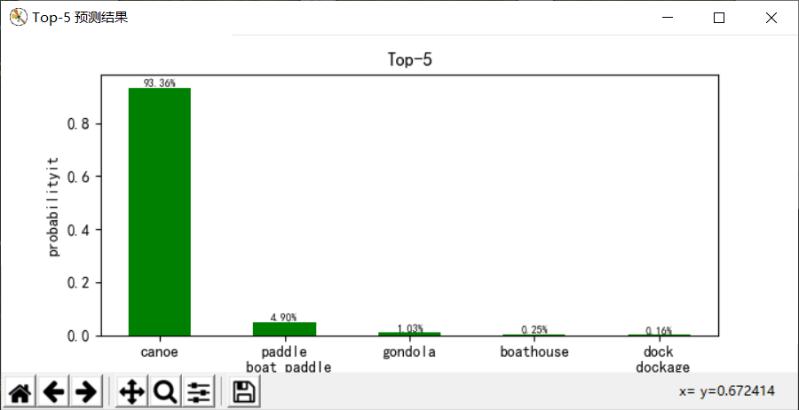
Type "help", "copyright", "credits" or "license()" for more information.
>>> 
 RESTART: G:\TestProject\...\vgg\app.py 
Input the path and image name:pic/8.jpg
path(vgg16.npy): G:\TestProject\...\vgg\vgg16.npy
key in data_dict: conv5_1
key in data_dict: fc6
key in data_dict: conv5_3
key in data_dict: conv5_2
key in data_dict: fc8
key in data_dict: fc7
key in data_dict: conv4_1
key in data_dict: conv4_2
key in data_dict: conv4_3
key in data_dict: conv3_3
key in data_dict: conv3_2
key in data_dict: conv3_1
key in data_dict: conv1_1
key in data_dict: conv1_2
key in data_dict: conv2_2
key in data_dict: conv2_1
build model started...
==>input image shape: [1, 224, 224, 3]
=>after conv1_1 shape: [1, 224, 224, 64]
=>after conv1_2 shape: [1, 224, 224, 64]
---after pool1 shape: [1, 112, 112, 64]
=>after conv2_1 shape: [1, 112, 112, 128]
=>after conv2_2 shape: [1, 112, 112, 128]
---after pool2 shape: [1, 56, 56, 128]
=>after conv3_1 shape: [1, 56, 56, 256]
=>after conv3_2 shape: [1, 56, 56, 256]
=>after conv3_3 shape: [1, 56, 56, 256]
---after pool3 shape: [1, 28, 28, 256]
=>after conv4_1 shape: [1, 28, 28, 512]
=>after conv4_2 shape: [1, 28, 28, 512]
=>after conv4_3 shape: [1, 28, 28, 512]
---after pool4 shape: [1, 14, 14, 512]
=>after conv5_1 shape: [1, 14, 14, 512]
=>after conv5_2 shape: [1, 14, 14, 512]
=>after conv5_3 shape: [1, 14, 14, 512]
---after pool5 shape: [1, 7, 7, 512]
fc_layer shape: [1, 7, 7, 512]
=>after fc6 shape: [1, 4096]
fc_layer shape: [1, 4096]
=>after fc7 shape: [1, 4096]
fc_layer shape: [1, 4096]
=>after fc8 shape: [1, 1000]
forward time consuming: 2.671326
top5 obj id: [472 693 576 449 536]
== top 1 ==
obj id: 472
--> canoe ---- 93.36%
== top 2 ==
obj id: 693
--> paddle
 boat paddle ---- 4.90%
== top 3 ==
obj id: 576
--> gondola ---- 1.03%
== top 4 ==
obj id: 449
--> boathouse ---- 0.25%
== top 5 ==
obj id: 536
--> dock
 dockage
 docking facility ---- 0.16%
>>> 

结果分析

选用这张小船的图片（/pic/8.jpg）进行测试，程序先加载训练模型参数文件（vgg16.npy），里面以字典形式保存网路参数（权重偏置等），可以打印显示键值名称，之后进行网络的前向传播，图片输入为：224x224x3，随着网络层数加深，数据尺寸不断减小，厚度不断增加，变为7x7x512后，被拉伸为1列数据，之后经过3层全连接层以及softmax分类输出，最终模型给出Top5预测结果，以93.36%的把握认为图片是canoe（独木舟，轻舟），4.90%的把握认为是paddle boat paddle（桨划船），预测效果还是不错的。

参考：人工智能实践：Tensorflow笔记