翻译自:waleedka/traffic-signs-tensorflow交通标识分类-tensorflow实现

首先引入必要的库

1
2
3
4
5
6
7
8
9
10
11
import os
import random
import skimage.data
import skimage.transform
import matplotlib
import matplotlib.pyplot as plt
import numpy as np
import tensorflow as tf

# Allow image embeding in notebook
%matplotlib inline

数据集解析

数据目录结构:

1
2
/traffic/datasets/BelgiumTS/Training/
/traffic/datasets/BelgiumTS/Testing/

训练集和测试集下分别有 62 个子目录,名字为 00000 to 00061。
目录的名称代表从0到61的标签,每个目录中的图像代表属于该标签的交通标志。
图片的存储格式为 .ppm 格式, 可以使用skimage library读取。

1
2
3
4
5
6
7
8
9
10
11
12
13
14
15
16
17
18
19
20
21
22
23
24
25
26
27
28
29
30
31
def load_data(data_dir):
"""Loads a data set and returns two lists:

images: a list of Numpy arrays, each representing an image.
labels: a list of numbers that represent the images labels.
"""
# Get all subdirectories of data_dir. Each represents a label.
directories = [d for d in os.listdir(data_dir)
if os.path.isdir(os.path.join(data_dir, d))]
# Loop through the label directories and collect the data in
# two lists, labels and images.
labels = []
images = []
for d in directories:
label_dir = os.path.join(data_dir, d)
file_names = [os.path.join(label_dir, f)
for f in os.listdir(label_dir) if f.endswith(".ppm")]
# For each label, load it's images and add them to the images list.
# And add the label number (i.e. directory name) to the labels list.
for f in file_names:
images.append(skimage.data.imread(f))
labels.append(int(d))
return images, labels


# Load training and testing datasets.
ROOT_PATH = ""
train_data_dir = os.path.join(ROOT_PATH, "datasets/BelgiumTS/Training")
test_data_dir = os.path.join(ROOT_PATH, "datasets/BelgiumTS/Testing")
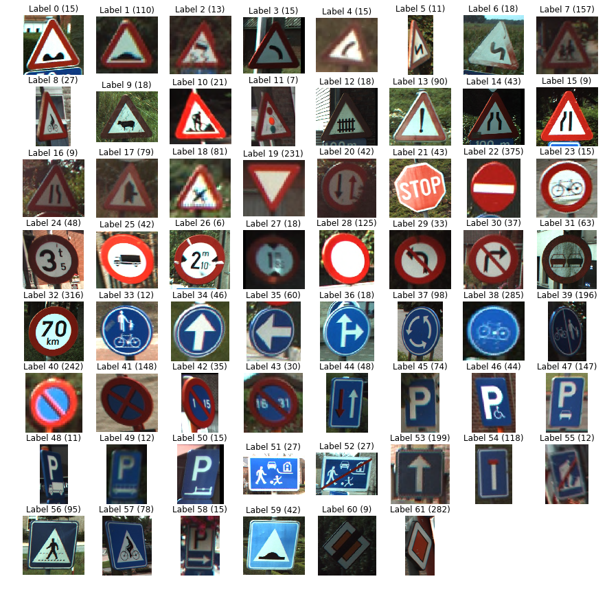
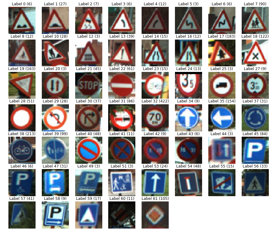
images, labels = load_data(train_data_dir)

打印出所有的图片和标签个数

1
print("Unique Labels: {0}\nTotal Images: {1}".format(len(set(labels)), len(images)))
1
2
Unique Labels: 62
Total Images: 4575

显示每类标签的第一个图片

1
2
3
4
5
6
7
8
9
10
11
12
13
14
15
16
17
18
def display_images_and_labels(images, labels):
"""Display the first image of each label."""
unique_labels = set(labels) # set:不重复出现
plt.figure(figsize=(15, 15)) # figure size
i = 1
for label in unique_labels:
# Pick the first image for each label.
image = images[labels.index(label)] #每个label在整个labels表中的位置
# str1.index(str2, beg=0, end=len(string)) str2在str1中的索引值
# print(labels.index(label))
plt.subplot(8, 8, i) # A grid of 8 rows x 8 columns
plt.axis('off')
plt.title("Label {0} ({1})".format(label, labels.count(label)))# label,totalnum
i += 1
_ = plt.imshow(image)
plt.show()
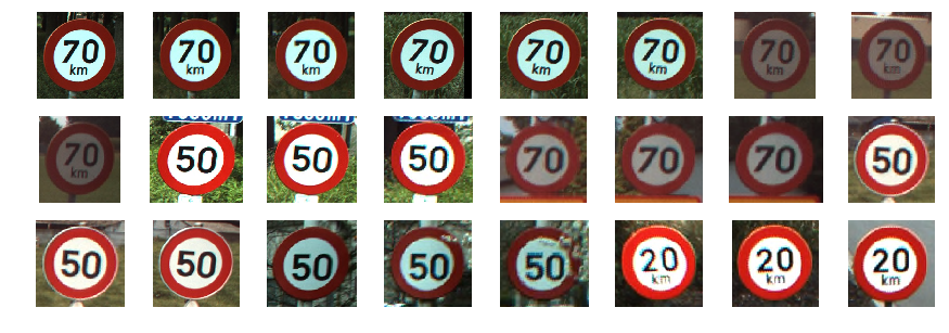
display_images_and_labels(images, labels)

mark

图片虽然是方形的,但是每一种图片的长宽比都不一样。而神经网络的输入大小是固定的,所以需要做一些处理工作。处理之前先拿一个标签图片出来,多看几张该标签下的图片,比如标签32,如下:

1
2
3
4
5
6
7
8
9
10
11
12
13
14
15
16
def display_label_images(images, label):
"""Display images of a specific label."""
limit = 24 # show a max of 24 images
plt.figure(figsize=(15, 5))
i = 1

start = labels.index(label)
end = start + labels.count(label)# count:统计字符串里某个字符出现的次数
for image in images[start:end][:limit]:
plt.subplot(3, 8, i) # 3 rows, 8 per row
plt.axis('off')
i += 1
plt.imshow(image)
plt.show()

display_label_images(images, 32)

mark

从上述图片中,我们可以发现虽然限速大小不同,但是都被归纳到同一类了。这非常好,后续的程序中,我们就可以忽略数字这个概念了。这就是为什么事先理解你的数据集是如此重要,可以在后续工作中为你节省很多的痛苦和混乱。

那么原始图片的大小到底是什么呢?让我们先来打印一些看看:
(小技巧:打印min()和max()值。这是一种简单的方法来验证您的数据的范围并及早发现错误)

1
2
for image in images[:5]:
print("shape: {0}, min: {1}, max: {2}".format(image.shape, image.min(), image.max()))
1
2
3
4
5
shape: (141, 142, 3), min: 0, max: 255
shape: (120, 123, 3), min: 0, max: 255
shape: (105, 107, 3), min: 0, max: 255
shape: (94, 105, 3), min: 7, max: 255
shape: (128, 139, 3), min: 0, max: 255

图片的尺寸大约在 128 * 128 左右,那么我们可以使用这个尺寸来保存图片,这样可以保存尽可能多的信息。但是,在早期的开发中,使用更小的尺寸,训练模型将很快,能够更快的迭代。
选择 32 * 32 的尺寸,这在肉眼下很容易识别图片(见下图),并且我们是要保证缩小的比例是 128 * 128 的倍数。

1
2
3
4
# Resize images
images32 = [skimage.transform.resize(image, (32, 32))
for image in images]
display_images_and_labels(images32, labels)

mark

32x32的图像不是那么清晰,但仍然可以辨认。请注意,上面的显示显示了大于实际大小的图像,因为matplotlib库试图将它们与网格大小相匹配。

下面打印一些图像的大小来验证我们是否正确。

1
2
for image in images32[:5]:
print("shape: {0}, min: {1}, max: {2}".format(image.shape, image.min(), image.max()))
1
2
3
4
5
shape: (32, 32, 3), min: 0.03529411764705882, max: 0.996078431372549
shape: (32, 32, 3), min: 0.033953737745098134, max: 0.996078431372549
shape: (32, 32, 3), min: 0.03694182751225489, max: 0.996078431372549
shape: (32, 32, 3), min: 0.06460056678921595, max: 0.9191425398284313
shape: (32, 32, 3), min: 0.06035539215686279, max: 0.9028492647058823

大小是正确的。但是请检查最小值和最大值!它们现在的范围从0到1.0,这与我们上面看到的0-255的范围不同。缩放函数为我们做了这个变换。将值标准化到0-1.0的范围非常普遍,所以我们会保留它。但是记住,如果你想要将图像转换回正常的0-255范围,要乘以255。

1
2
3
labels_a = np.array(labels) # 标签
images_a = np.array(images32) # 图片
print("labels: ", labels_a.shape, "\nimages: ", images_a.shape)
1
2
labels:  (4575,) 
images: (4575, 32, 32, 3)

模型建立

首先创建一个Graph对象。

然后设置了占位符(Placeholder)用来放置图片和标签。占位符是TensorFlow从主程序中接收输入的方式。
参数 images_ph 的维度是 [None, 32, 32, 3],这四个参数分别表示 [批量大小,高度,宽度,通道] (通常缩写为 NHWC)。批处理大小用 None 表示,意味着批处理大小是灵活的,也就是说,可以向模型中导入任意批量大小的数据,而不用去修改代码。

全连接层的输出是一个长度是62的对数矢量。输出的数据可能看起来是这样的:[0.3, 0, 0, 1.2, 2.1, 0.01, 0.4, … …, 0, 0]。值越高,图片越可能表示该标签。输出的不是一个概率,他们可以是任意的值,并且相加的结果不等于1。输出神经元的实际值大小并不重要,因为这只是一个相对值,相对62个神经元而言。如果需要,我们可以很容易的使用 softmax 函数或者其他的函数转换成概率(这里不需要)。

在这个项目中,只需要知道最大值所对应的索引就行了,因为这个索引代表着图片的分类标签。argmax 函数的输出结果将是一个整数,范围是 [0, 61]。

损失函数采用交叉熵计算方法,因为交叉熵更适合分类问题,而平方差适合回归问题。
交叉熵是两个概率向量之间的差的度量。因此,我们需要将标签和神经网络的输出转换成概率向量。TensorFlow中有一个 sparse_softmax_cross_entropy_with_logits 函数可以实现这个操作。这个函数将标签和神经网络的输出作为输入参数,并且做三件事:第一,将标签的维度转换为 [None, 62](这是一个0-1向量);第二,利用softmax函数将标签数据和神经网络输出结果转换成概率值;第三,计算两者之间的交叉熵。这个函数将会返回一个维度是 [None] 的向量(向量长度是批处理大小),然后我们通过 reduce_mean 函数来获得一个值,表示最终的损失值。

模型参数的调整选用梯度下降算法,经试验学习率选用0.08比较合适,迭代800次。

1
2
3
4
5
6
7
8
9
10
11
12
13
14
15
16
17
18
19
20
21
22
23
24
25
26
27
28
29
30
31
32
33
34
35
36
37
# Create a graph to hold the model.
graph = tf.Graph()

# Create model in the graph.
with graph.as_default():
# Placeholders for inputs and labels.
images_ph = tf.placeholder(tf.float32, [None, 32, 32, 3])
labels_ph = tf.placeholder(tf.int32, [None])

# Flatten input from: [None, height, width, channels]
# To: [None, height * width * channels] == [None, 3072]
images_flat = tf.contrib.layers.flatten(images_ph)

# Fully connected layer. 【全连接层】
# Generates logits of size [None, 62]
logits = tf.contrib.layers.fully_connected(images_flat, 62, tf.nn.relu)

# Convert logits to label indexes (int).
# Shape [None], which is a 1D vector of length == batch_size.
predicted_labels = tf.argmax(logits, 1)

# Define the loss function. 【损失函数】
# Cross-entropy is a good choice for classification. 交叉熵
loss = tf.reduce_mean(tf.nn.sparse_softmax_cross_entropy_with_logits(logits=logits, labels=labels_ph))

# Create training op. 【梯度下降算法】
train = tf.train.GradientDescentOptimizer(learning_rate=0.08).minimize(loss)

# And, finally, an initialization op to execute before training.
# TODO: rename to tf.global_variables_initializer() on TF 0.12.
init = tf.global_variables_initializer()

print("images_flat: ", images_flat)
print("logits: ", logits)
print("loss: ", loss)
print("predicted_labels: ", predicted_labels)
print(tf.nn.sparse_softmax_cross_entropy_with_logits(logits=logits, labels=labels_ph))
1
2
3
4
5
images_flat:  Tensor("Flatten/flatten/Reshape:0", shape=(?, 3072), dtype=float32)
logits: Tensor("fully_connected/Relu:0", shape=(?, 62), dtype=float32)
loss: Tensor("Mean:0", shape=(), dtype=float32)
predicted_labels: Tensor("ArgMax:0", shape=(?,), dtype=int64)
Tensor("SparseSoftmaxCrossEntropyWithLogits_1/SparseSoftmaxCrossEntropyWithLogits:0", shape=(?,), dtype=float32)

训练

1
2
3
4
5
6
# Create a session to run the graph we created.
session = tf.Session(graph=graph)

# First step is always to initialize all variables.
# We don't care about the return value, though. It's None.
_ = session.run([init])
1
2
3
4
5
for i in range(801):
_, loss_value = session.run([train, loss],
feed_dict={images_ph: images_a, labels_ph: labels_a})
if i % 20 == 0:
print("Loss: ", loss_value)
1
2
3
4
5
6
7
8
9
10
11
12
13
14
15
16
17
18
19
20
21
22
23
24
25
26
27
28
29
30
31
32
33
34
35
36
37
38
39
40
41
Loss:  4.237691
Loss: 3.4573376
Loss: 3.081502
Loss: 2.89802
Loss: 2.780877
Loss: 2.6962612
Loss: 2.6338725
Loss: 2.5843806
Loss: 2.5426073
Loss: 2.5067272
Loss: 2.47533
Loss: 2.4474416
Loss: 2.4224002
Loss: 2.399726
Loss: 2.3790603
Loss: 2.360102
Loss: 2.3426225
Loss: 2.3264341
Loss: 2.3113735
Loss: 2.2973058
Loss: 2.2841291
Loss: 2.2717524
Loss: 2.2600884
Loss: 2.248851
Loss: 2.2366288
Loss: 2.2220945
Loss: 2.2083163
Loss: 2.1957521
Loss: 2.184217
Loss: 2.1736012
Loss: 2.1637862
Loss: 2.1546829
Loss: 2.1461952
Loss: 2.1382334
Loss: 2.13073
Loss: 2.1236277
Loss: 2.1168776
Loss: 2.1104405
Loss: 2.104286
Loss: 2.0983875
Loss: 2.0927253

使用训练的模型-测试训练集上的准确率

会话对象(session)包含模型中所有变量的值(即权重)。

1
2
3
4
5
6
7
8
9
10
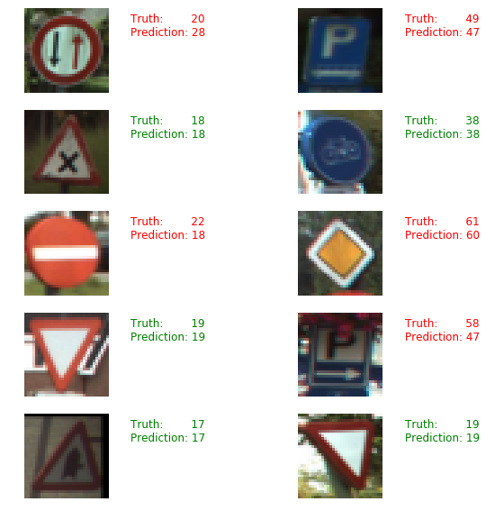
# 随机从训练集中选取10张图片
sample_indexes = random.sample(range(len(images32)), 10)
sample_images = [images32[i] for i in sample_indexes]
sample_labels = [labels[i] for i in sample_indexes]

# Run the "predicted_labels" op.
predicted = session.run([predicted_labels],
feed_dict={images_ph: sample_images})[0]
print(sample_labels)#样本标签
print(predicted)#预测值
1
2
[20, 49, 18, 38, 22, 61, 19, 58, 17, 19]
[28 47 18 38 18 60 19 47 17 19]
1
2
3
4
5
6
7
8
9
10
11
12
# Display the predictions and the ground truth visually.
fig = plt.figure(figsize=(10, 10))
for i in range(len(sample_images)):
truth = sample_labels[i]
prediction = predicted[i]
plt.subplot(5, 2,1+i)
plt.axis('off')
color='green' if truth == prediction else 'red'
plt.text(40, 10, "Truth: {0}\nPrediction: {1}".format(truth, prediction),
fontsize=12, color=color)
plt.imshow(sample_images[i])

mark

上图truth后的数字为真实的标签,Prediction后的数字为预测的标签。
现在的分类测试还是训练集中的图片,所以还不知道模型在未知数据集上面的效果如何。
接下来在测试集上面进行评测。

模型评估-验证测试集上的准确率

可视化结果很直观,但是需要更精确的方法来测量模型的准确性,这就是验证集发挥作用的地方。

1
2
# 加载测试集图片
test_images, test_labels = load_data(test_data_dir)
1
2
3
4
5
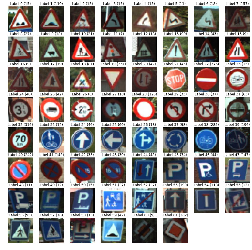
# 转换图片尺寸
test_images32 = [skimage.transform.resize(image, (32, 32))
for image in test_images]
#显示转换后的图片
display_images_and_labels(test_images32, test_labels)

mark

1
2
3
4
5
6
7
8
# Run predictions against the full test set.
predicted = session.run([predicted_labels],
feed_dict={images_ph: test_images32})[0]
# 计算准确度
match_count = sum([int(y == y_) for y, y_ in zip(test_labels, predicted)])
accuracy = match_count / len(test_labels)
# 输出测试集上的准确度
print("Accuracy: {:.3f}".format(accuracy))
1
Accuracy: 0.534
1
2
# Close the session. This will destroy the trained model.
session.close()